Contents

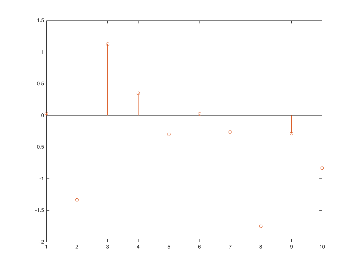
compare inverse DFS and original signal

figure
x = randn(1,10);
stem(x);
X=dfs(x,10);
x1 = idfs(X,10);
hold on;
stem(real(x1));

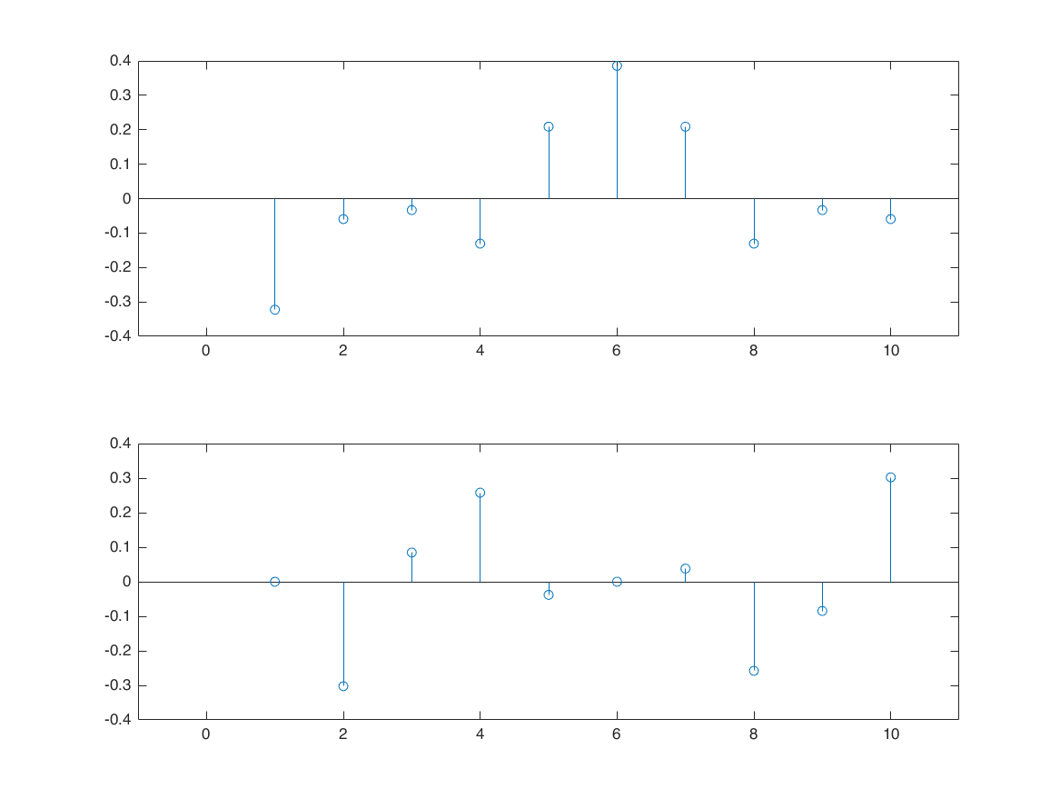
figure
subplot(2,1,1)
stem(real(X)); xlim([-1,11])
subplot(2,1,2)
stem(imag(X)); xlim([-1,11])

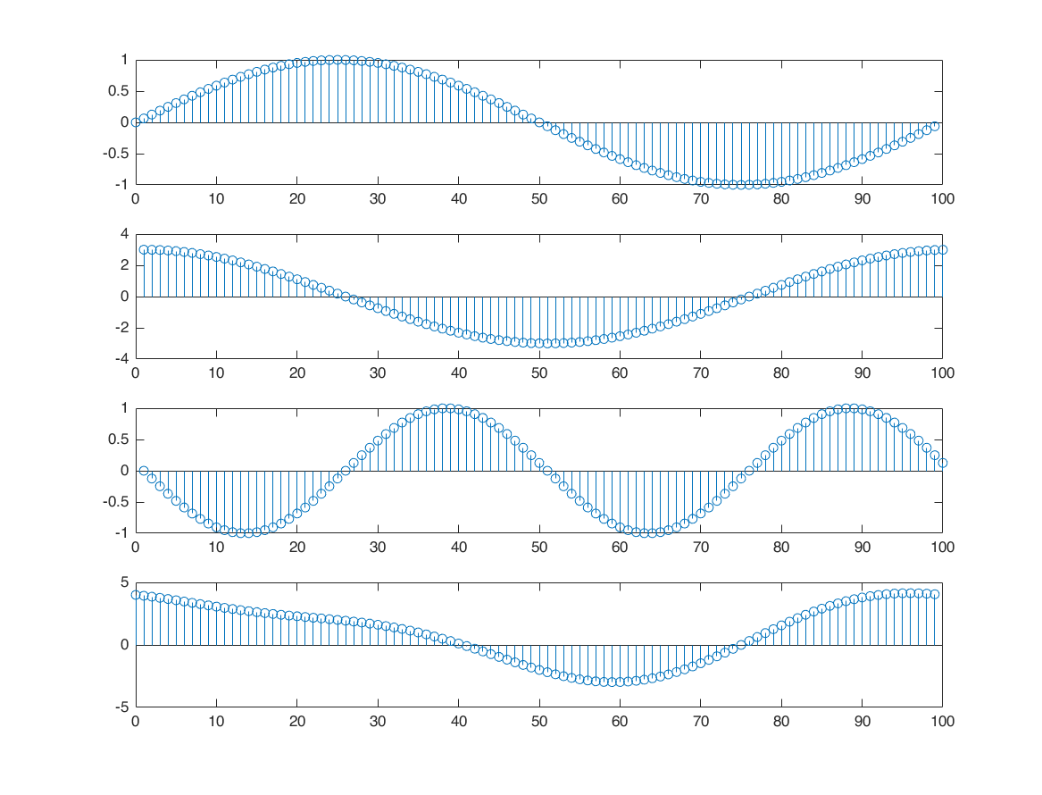
DSF example with sine waves

N = 100;
n = 0:1:N-1;
x = 1+sin(2*pi*n/N)+3*cos(2*pi*n/N)+cos(4*pi*n/N+pi/2);
figure
subplot(4,1,1); stem(n,sin(2*pi*n/N));
subplot(4,1,2); stem(3*cos(2*pi*n/N))
subplot(4,1,3); stem(cos(4*pi*n/N+pi/2))
subplot(4,1,4); stem(n,x)

X = dfs(x,N);

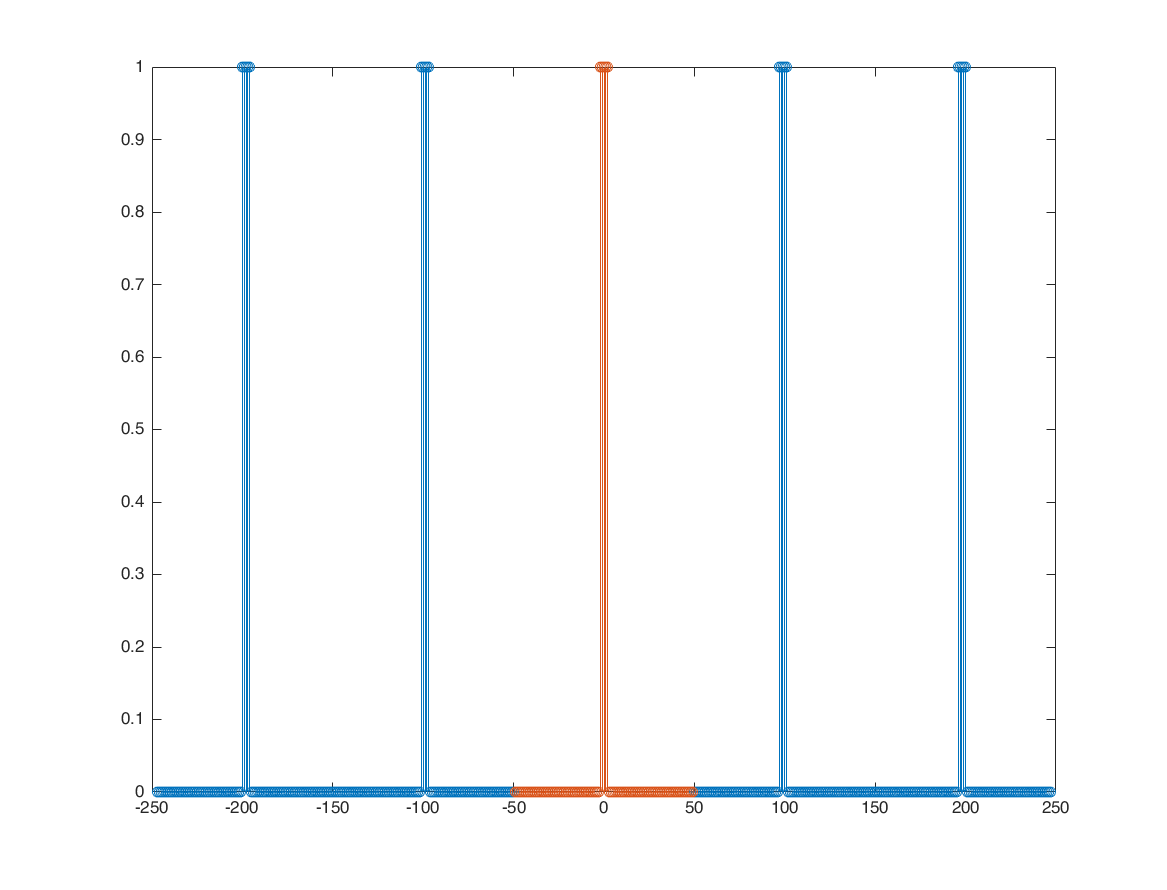
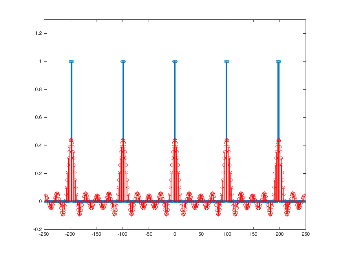
square wave train (periodic in time)

periodic square train

N = 99; % 11 17 41 73
N1 = 2;

x0 = zeros([1 N]);
nx0 = -(N-1)/2:1:(N-1)/2;
x0(abs(nx0)<=N1) = 1;
x = repmat(x0, 1, 5);
nx = -(length(x)-1)/2:1:(length(x)-1)/2;

figure
stem(nx,x); hold on;
stem(nx0,x0)

% calculate DSF with DFS analysis formula
k = nx0;
a = x0*exp(-1i*2*pi/N*k'*nx0)/N;

% calculate DFS with analytical method
O = 2*pi*k/N;
b = sin((2*N1+1)*O/2)./sin(O/2)/N;
b(isnan(b)) = (2*N1+1)/N;

figure
stem(O,real(a)*N); hold on;
stem(O,N*b)

%       you can increase N and see the effect. When we have N=9, we have 9
% sample in frequency domain. When we have N=11, we get 11 sample in
% frequency domain, and etc.

%       Rule of thumb: Increasing N in time gives you denser sample in fequency.
% this is apparent because Omega is getting denser. At the same time, k
% change and is from -(N-1)/2 to (N-1)/2 (length=N).

%       Base on above: What happen if you increase N to infinity?
% answer: the time axis becomes so dense that we get a continuous function.
% Here we can see how time and frequency axis can be related! Increasing
% the period in the time domain == increasing the number of samples (denser
% frequency axis) in frequency domain. As long as the shape of one period
% not change in time, the frequncy shape will not change.

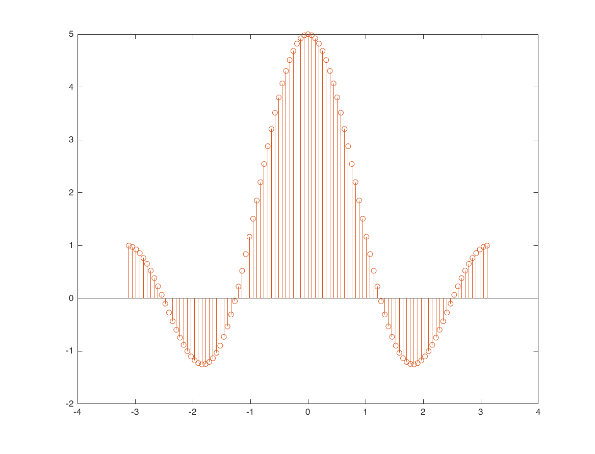
synthensis formula

c = (N-1)/2+1;

k = 0;
x0 = a(c+k)*exp(1i*k*(2*pi/N)*nx);

figure
stem(nx,x); ylim([-0.2,1.3]); hold on;
stem(nx,real(x0),'r'); hold off;

pause(1)

k = 1;
x1 = x0 + a(c+k)*exp(1i*k*(2*pi/N)*nx);

k = -1;
x1 = x1 + a(c+k)*exp(1i*k*(2*pi/N)*nx);

stem(nx,x); ylim([-0.2,1.3]); hold on;
stem(nx,real(x1),'r'); hold off;

pause(1)

k = 2;
x2 = x1 + a(c+k)*exp(1i*k*(2*pi/N)*nx);

k = -2;
x2 = x2 + a(c+k)*exp(1i*k*(2*pi/N)*nx);

stem(nx,x); ylim([-0.2,1.3]); hold on;
stem(nx,real(x2),'r'); hold off;

pause(1)

k = 3;
x3 = x2 + a(c+k)*exp(1i*k*(2*pi/N)*nx);

k = -3;
x3 = x3 + a(c+k)*exp(1i*k*(2*pi/N)*nx);

stem(nx,x); ylim([-0.2,1.3]); hold on;
stem(nx,real(x3),'r'); hold off;

pause(1)

k = 4;
x4 = x3 + a(c+k)*exp(1i*k*(2*pi/N)*nx);

k = -4;
x4 = x4 + a(c+k)*exp(1i*k*(2*pi/N)*nx);

stem(nx,x); ylim([-0.2,1.3]); hold on;
stem(nx,real(x4),'r'); hold off;

%       a fun fact: because the frequency is descrete, we don't see
% the Gibbs phenomenon. The gibbs happen when the frequency axis is
% continuous and we can't capture and synthesize all of the frequency
% components from the frequency domain to the time domain.
%       Here, because the frequency is descrete, we were able to eventually
% return all of the frequency components from frequency domain to the time
% domain.

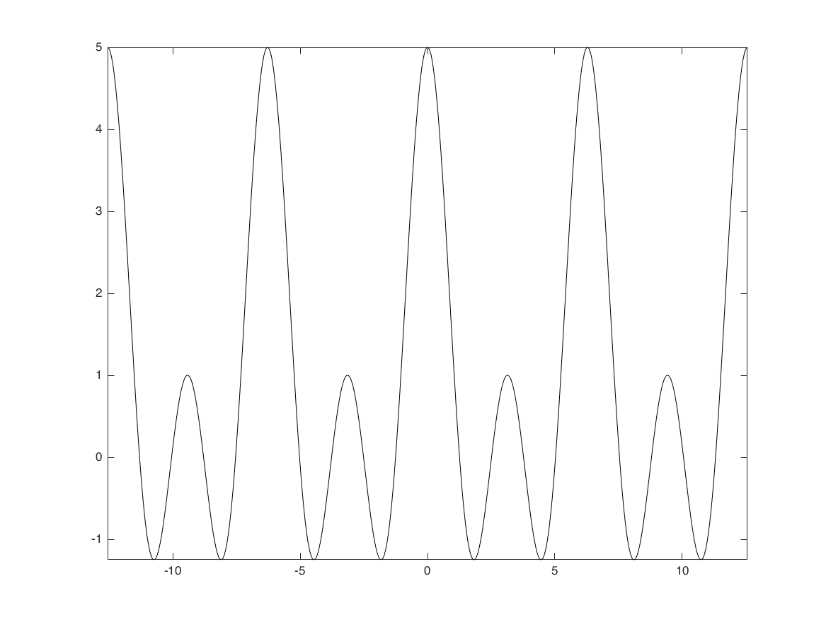
Aperiodic Square Wave

N1 = 2;

Omega = -4*pi:0.01:4*pi;
X = sin((2*N1+1)*Omega/2)./sin(Omega/2);

figure
plot(Omega,X,'k'); axis tight;

Published with MATLAB® R2016b