Contents

clc; clear; close all;

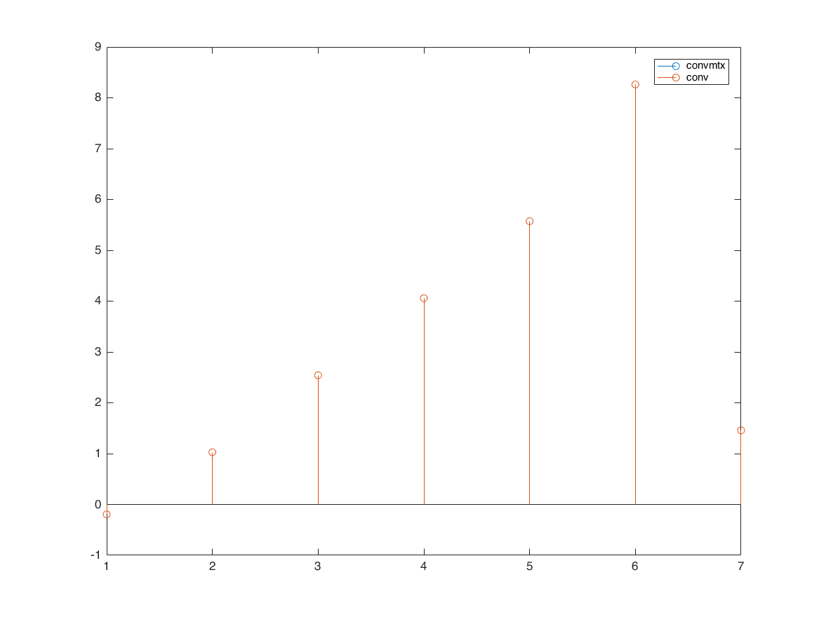
express convolution as matrix multiplication

h = [1 2 3 4 5]';
x = randn(3,1);
A = convmtx(h,length(x));
y = A*x;
y1 = conv(h,x);
figure
stem(y)
hold on
stem(y1)
legend('convmtx','conv')

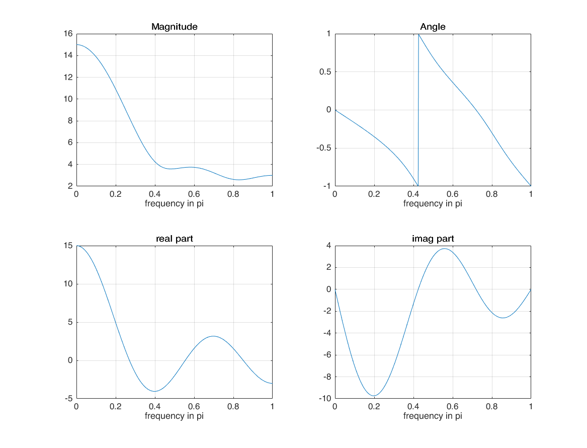
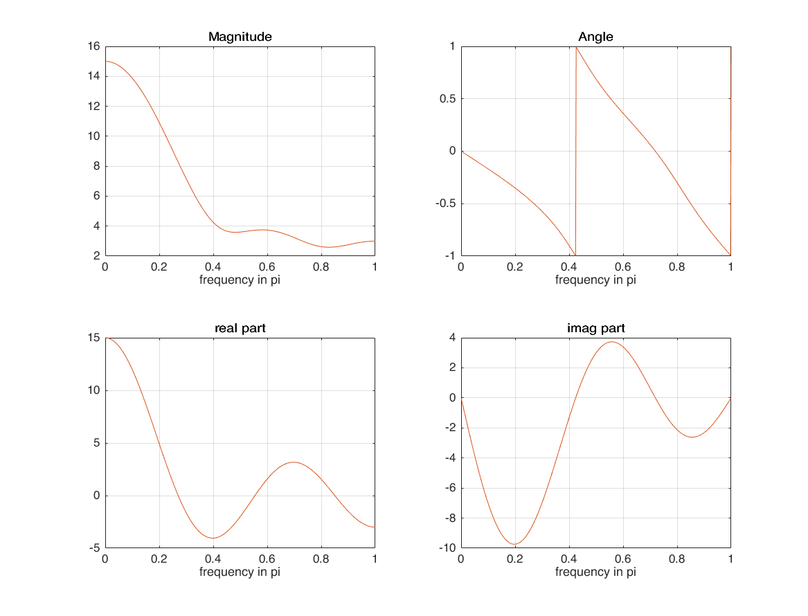
matlab DTFT implementation

n = -1:3;
x = 1:5;

M = 500;
k = 0:M;
w = (pi/M)*k;

X = x * (exp(-1i*pi/M)).^(n'*k);

magX = abs(X);
angX = angle(X);
realX = real(X);
imagX = imag(X);

subplot(2,2,1); plot(k/M, magX); grid on;
xlabel('frequency in pi'); title('Magnitude');

subplot(2,2,2); plot(k/M, angX/pi); grid on;
xlabel('frequency in pi'); title('Angle');

subplot(2,2,3); plot(k/M, realX); grid on;
xlabel('frequency in pi'); title('real part');

subplot(2,2,4); plot(k/M, imagX); grid on;
xlabel('frequency in pi'); title('imag part');

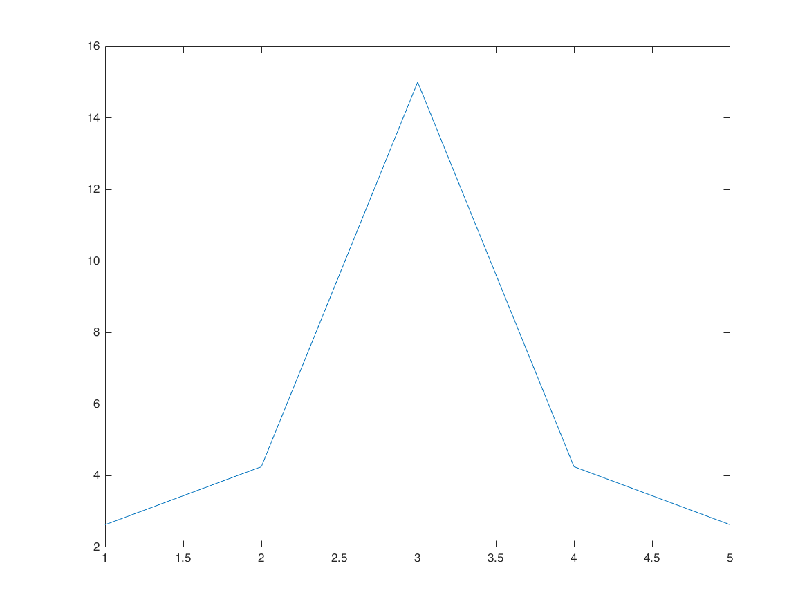
xf = fft(x);

figure
plot(abs(fftshift(xf)))

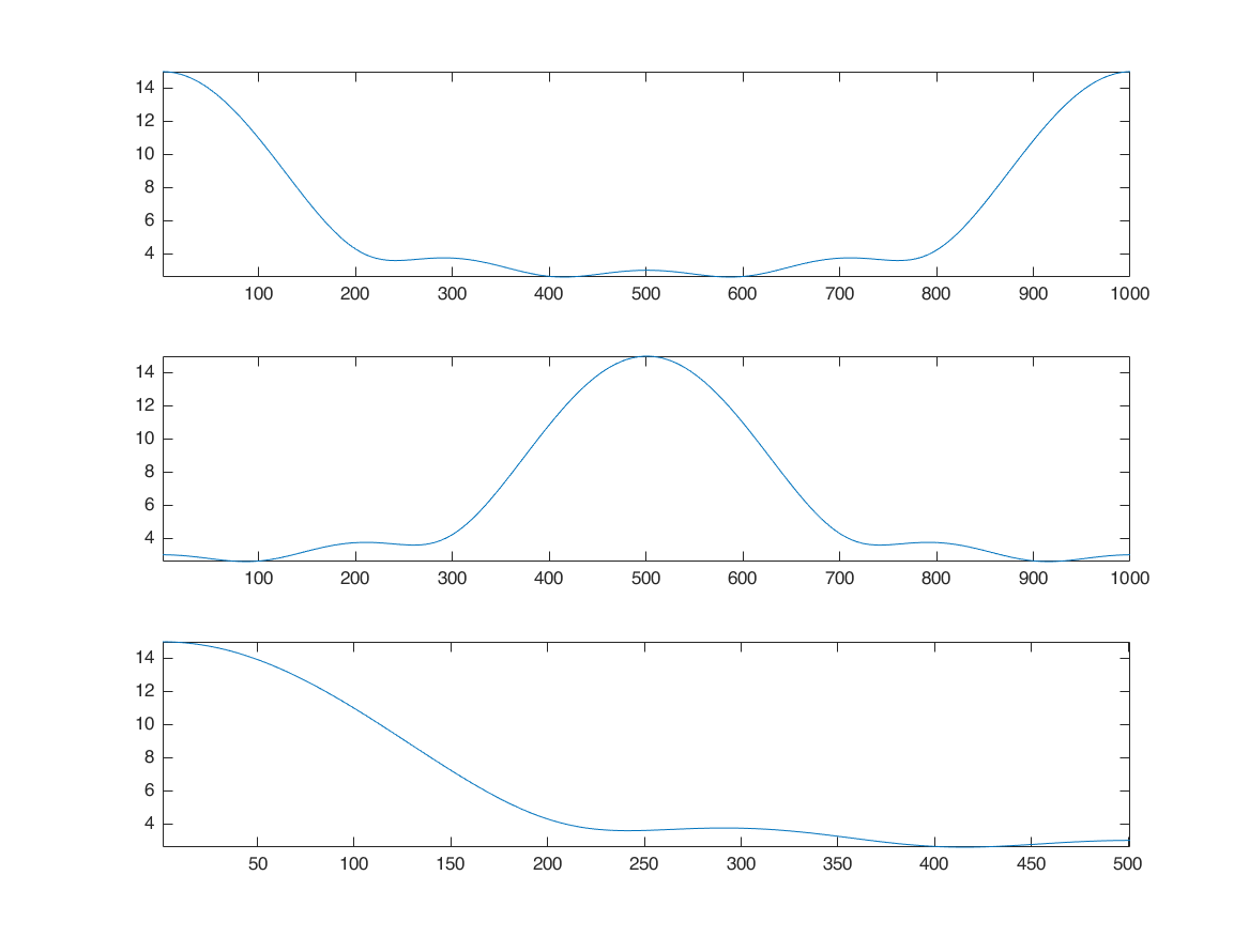
padding zero after array in time domain, densifies fft in frequency domain

remember: frequency output of fft is 0 to 2pi. to shift it and align zero frequency at the center, we use fftshift

x1 = zeros([M*2,1]);
x1(1:length(x)) = x;
xf = fft(x1);

figure
subplot(3,1,1); plot(abs(xf)); axis tight;
subplot(3,1,2); plot(abs(fftshift(xf))); axis tight;
subplot(3,1,3); plot(abs(xf(1:501))); axis tight;

compare angle of our own DFT and matlab's fft

figure
plot(k/M, realX); grid on; hold on;
plot(k/M, real(xf(1:length(X))), 'r')
xlabel('frequency in pi'); title('Angle');
legend(['real part of our own DFT function'],['real part of MATLAB FFT'])

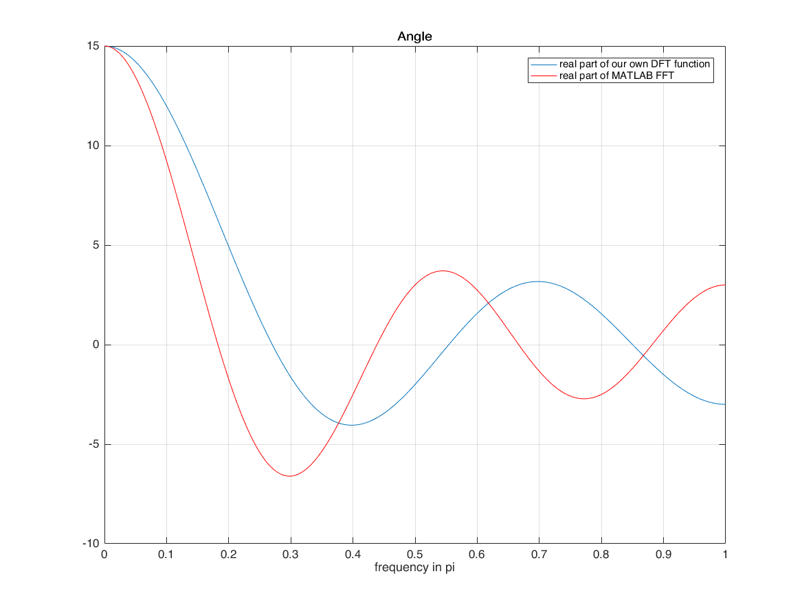
compare real and imag part of our own DFT and matlab's fft

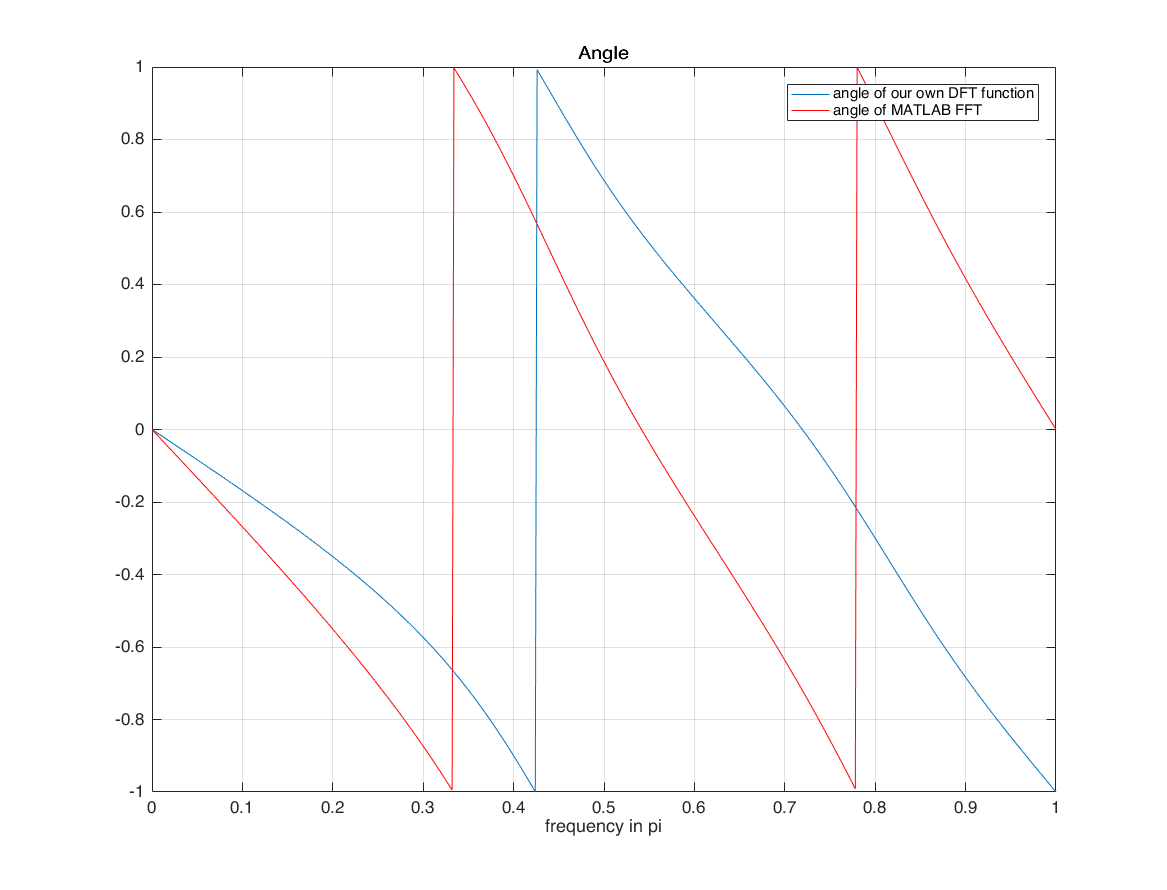
they are different because of the horizontal axis! horizontal axis of input is n=-1:3 we use horizontal axis when calculating X we did not use it with matlab FFT matlab assumes that horizontal axis of signal starts from 0! with time shifting property of DFT (DTFT), we can overcome this limitation

figure
plot(k/M, angX/pi); grid on; hold on;
plot(k/M, angle(xf(1:length(X)))/pi, 'r')
xlabel('frequency in pi'); title('Angle');
legend(['angle of our own DFT function'],['angle of MATLAB FFT'])

calculate fft of a signal that is not started from 0 ( for example started from -1 )

amount_of_shift = -1;
xf1 = xf(1:length(X)) .* exp(-1i*w'*(amount_of_shift));

figure
subplot(2,2,1); plot(k/M, magX); grid on; hold on;
plot(k/M, abs(xf1))
xlabel('frequency in pi'); title('Magnitude');

subplot(2,2,2); plot(k/M, angX/pi); grid on; hold on;
plot(k/M, angle(xf1)/pi)
xlabel('frequency in pi'); title('Angle');

subplot(2,2,3); plot(k/M, realX); grid on; hold on;
plot(k/M, real(xf1))
xlabel('frequency in pi'); title('real part');

subplot(2,2,4); plot(k/M, imagX); grid on; hold on;
plot(k/M, imag(xf1))
xlabel('frequency in pi'); title('imag part');

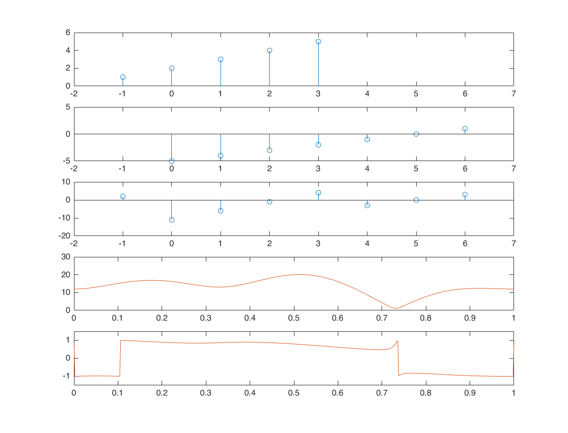
Linearity

n1 = -1:3;
x1 = 1:5;
alpha = 2;
xx1 = alpha*x1;

n2 = 0:6;
x2 = -5:1;
beta = 3;
xx2 = beta*x2;

[xx3,n3] = sigadd(xx1,n1,xx2,n2);

M = 500; %501 samples
k = 0:M;
w = (pi/M)*k;

X1 = x1*(exp(-1i*pi/M)).^(n1'*k);
X2 = x2*(exp(-1i*pi/M)).^(n2'*k);
X3 = xx3*(exp(-1i*pi/M)).^(n3'*k);
XX3 = alpha*X1 + beta*X2;

subplot(5,1,1); stem(n1,x1); xlim([-2 7]);
subplot(5,1,2); stem(n2,x2); xlim([-2 7]);
subplot(5,1,3); stem(n3,xx3); xlim([-2 7]);
subplot(5,1,4); plot(k/M, abs(X3)); hold on; plot(k/M, abs(XX3));
subplot(5,1,5); plot(k/M, angle(X3)/pi); hold on; plot(k/M, angle(XX3)/pi); ylim([-1.5,1.5]);

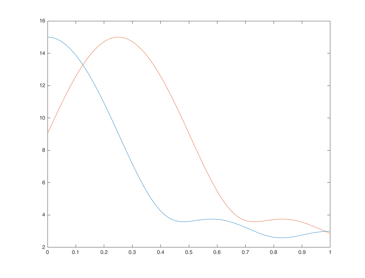
Frequency-shifting (modulation) - example 1

n1 = -1:3;
x1 = 1:5;
w0 = pi/4;

x2 = x1 .* exp(1i*w0*n1);

X1 = x1*(exp(-1i*pi/M)).^(n1'*k);
X2 = x2*(exp(-1i*pi/M)).^(n1'*k);

figure
plot(k/M, abs(X1)); hold on;
plot(k/M, abs(X2))

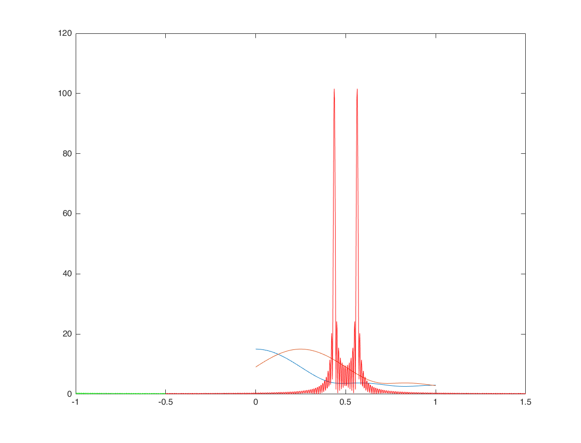
Frequency-shifting (modulation) - example 2

n = -100:100;
x = cos(0.2*n);

x1 = x.*exp(1i*pi/2*n); % modulated signal

M = 500;
k = -M:M;
w = (pi/M)*k;

X = x*(exp(-1i*pi/M)).^(n'*k);
X1 = x1*(exp(-1i*pi/M)).^(n'*k);

[XX1,F1] = sigshift(X,w,pi/2);

 hold on;
plot(k/M, abs(X1),'g')
plot(F1/pi, abs(XX1),'r')

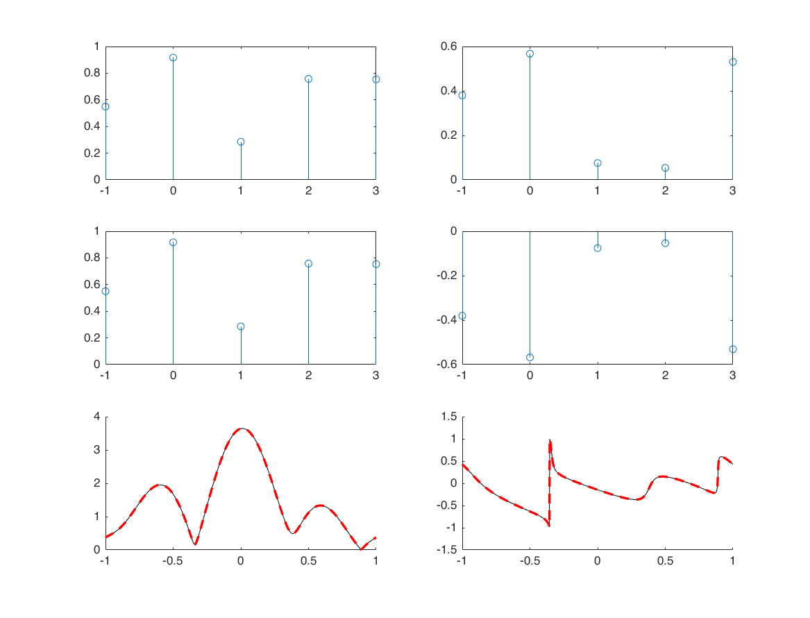
conjugation

n = -1:3;
x = rand(1,5)+1i*rand(1,5);
x1=conj(x);

figure
subplot(3,2,1); stem(n,real(x))
subplot(3,2,2); stem(n,imag(x))
subplot(3,2,3); stem(n,real(x1))
subplot(3,2,4); stem(n,imag(x1))

M = 500;
k = -M:M;
w = (pi/M)*k;

X = x*(exp(-1i*pi/M)).^(n'*k);
X1 = x1*(exp(-1i*pi/M)).^(n'*k);

XX1 = conj(sigfold(X,w));
subplot(3,2,5); hold on; plot(k/M, abs(X1),'k'); plot(k/M, abs(XX1),'r--','linewidth',2);
subplot(3,2,6); hold on; plot(k/M, angle(X1)/pi,'k'); plot(k/M, angle(XX1)/pi,'r--','linewidth',2); ylim([-1.5;1.5]);

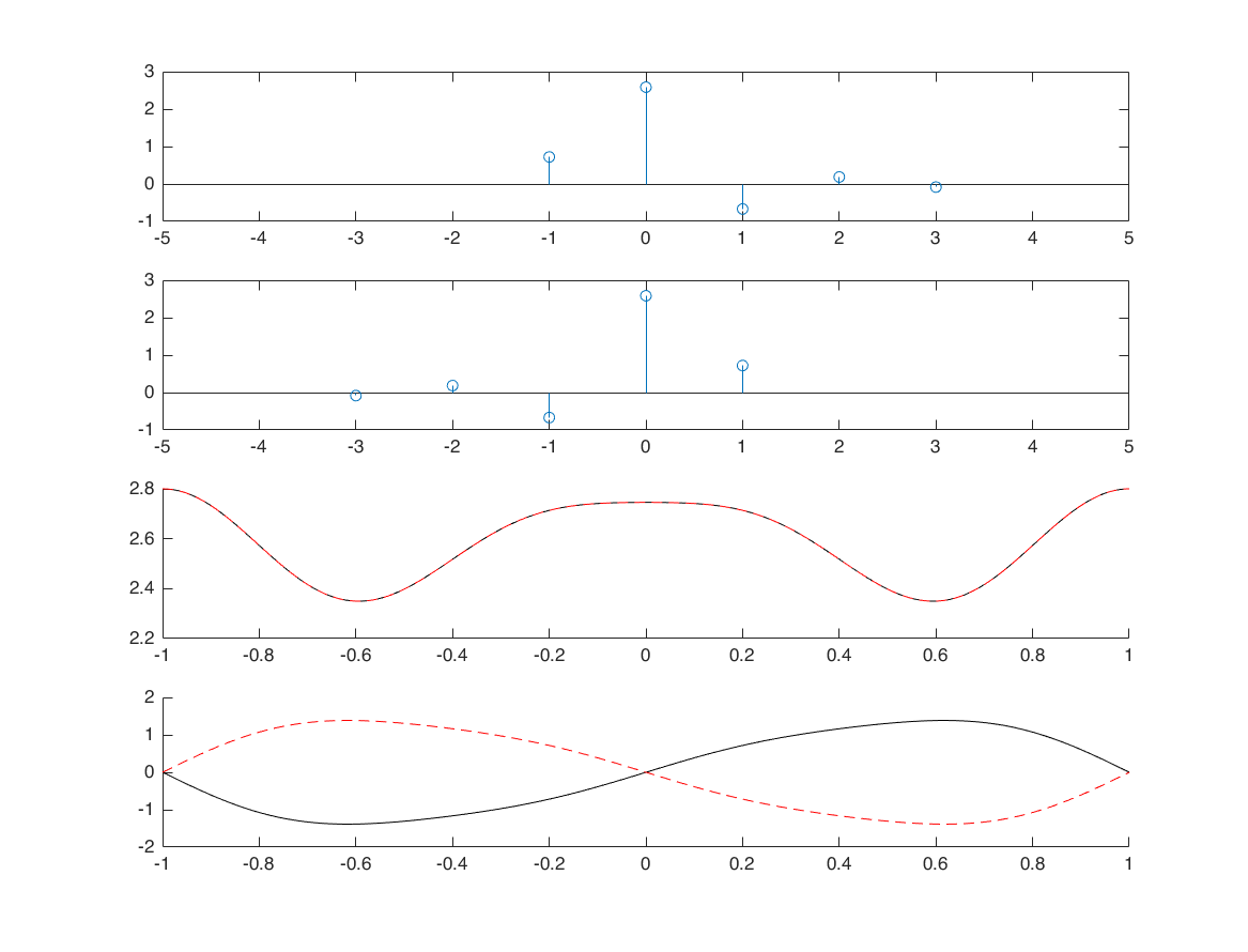
folding

nx = -1:3;
x = randn(1,5);
[x1,nx1] = sigfold(x,nx);

M = 500;
k = -M:M;
w = (pi/M)*k;

X = x*(exp(-1i*pi/M)).^(nx'*k);
X1 = x1*(exp(-1i*pi/M)).^(nx1'*k);

subplot(4,1,1)
stem(nx,x); xlim([-5 5])

subplot(4,1,2)
stem(nx1,x1); xlim([-5 5])

subplot(4,1,3); hold on;
plot(w/pi, real(X), 'k')
plot(w/pi, real(X1), 'r--')

subplot(4,1,4); hold on;
plot(w/pi, imag(X), 'k')
plot(w/pi, imag(X1), 'r--')

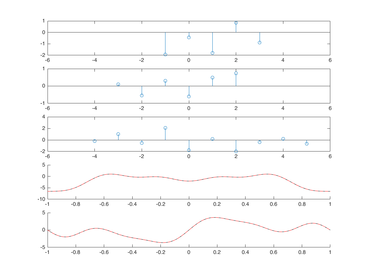
convolution

nx1 = -1:3;
x1 = randn([1 5]);
nx2 = -3:2;
x2 = randn([1 6]);
[x3, nx3] = conv_m(x1,nx1,x2,nx2);

M = 500;
k = -M:M;
w = (pi/M)*k;

X1 = x1*(exp(-1i*pi/M)).^(nx1'*k);
X2 = x2*(exp(-1i*pi/M)).^(nx2'*k);
X3 = x3*(exp(-1i*pi/M)).^(nx3'*k);
XX3 = X1.*X2;

figure
subplot(5,1,1); stem(nx1,x1); xlim([-6 6]);
subplot(5,1,2); stem(nx2,x2); xlim([-6 6]);
subplot(5,1,3); stem(nx3,x3); xlim([-6,6]);

subplot(5,1,4); hold on;
plot(w/pi, real(X3), 'k')
plot(w/pi, real(XX3), 'r--')

subplot(5,1,5); hold on;
plot(w/pi, imag(X3), 'k')
plot(w/pi, imag(XX3), 'r--')

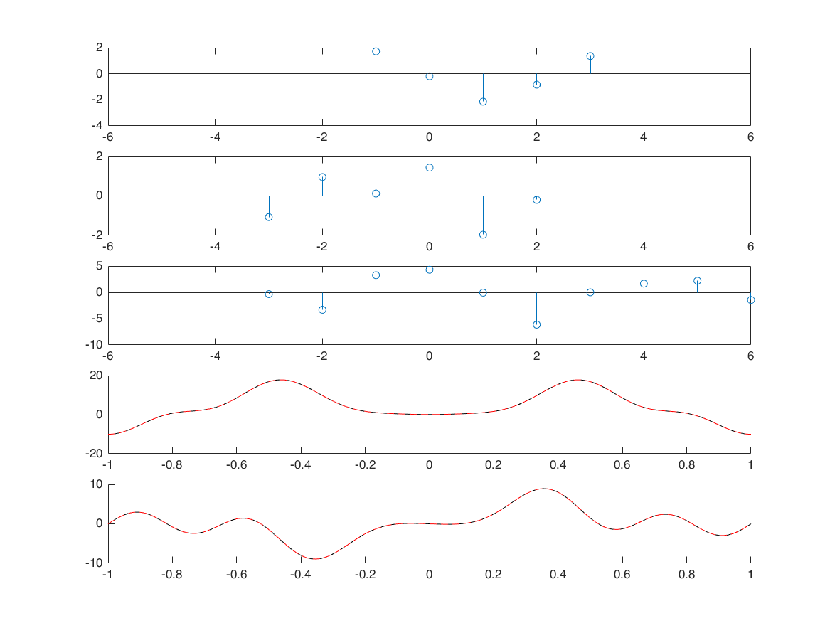
correlation

nx1 = -1:3;
x1 = randn([1 5]);
nx2 = -3:2;
x2 = randn([1 6]);
[x3, nx3] = xcorr_m(x1,nx1,x2,nx2);

% define frequency axis
M = 500;
k = -M:M;
w = (pi/M)*k;

X1 = x1*(exp(-1i*pi/M)).^(nx1'*k);
X2 = x2*(exp(-1i*pi/M)).^(nx2'*k);
X3 = x3*(exp(-1i*pi/M)).^(nx3'*k);
XX3 = X1.*conj(X2);

figure;
subplot(5,1,1); stem(nx1,x1); xlim([-6 6]);
subplot(5,1,2); stem(nx2,x2); xlim([-6 6]);
subplot(5,1,3); stem(nx3,x3); xlim([-6 6]);

subplot(5,1,4); hold on;
plot(w/pi, real(X3), 'k');
plot(w/pi, real(XX3), 'r--');

subplot(5,1,5); hold on;
plot(w/pi, imag(X3), 'k');
plot(w/pi, imag(XX3), 'r--');

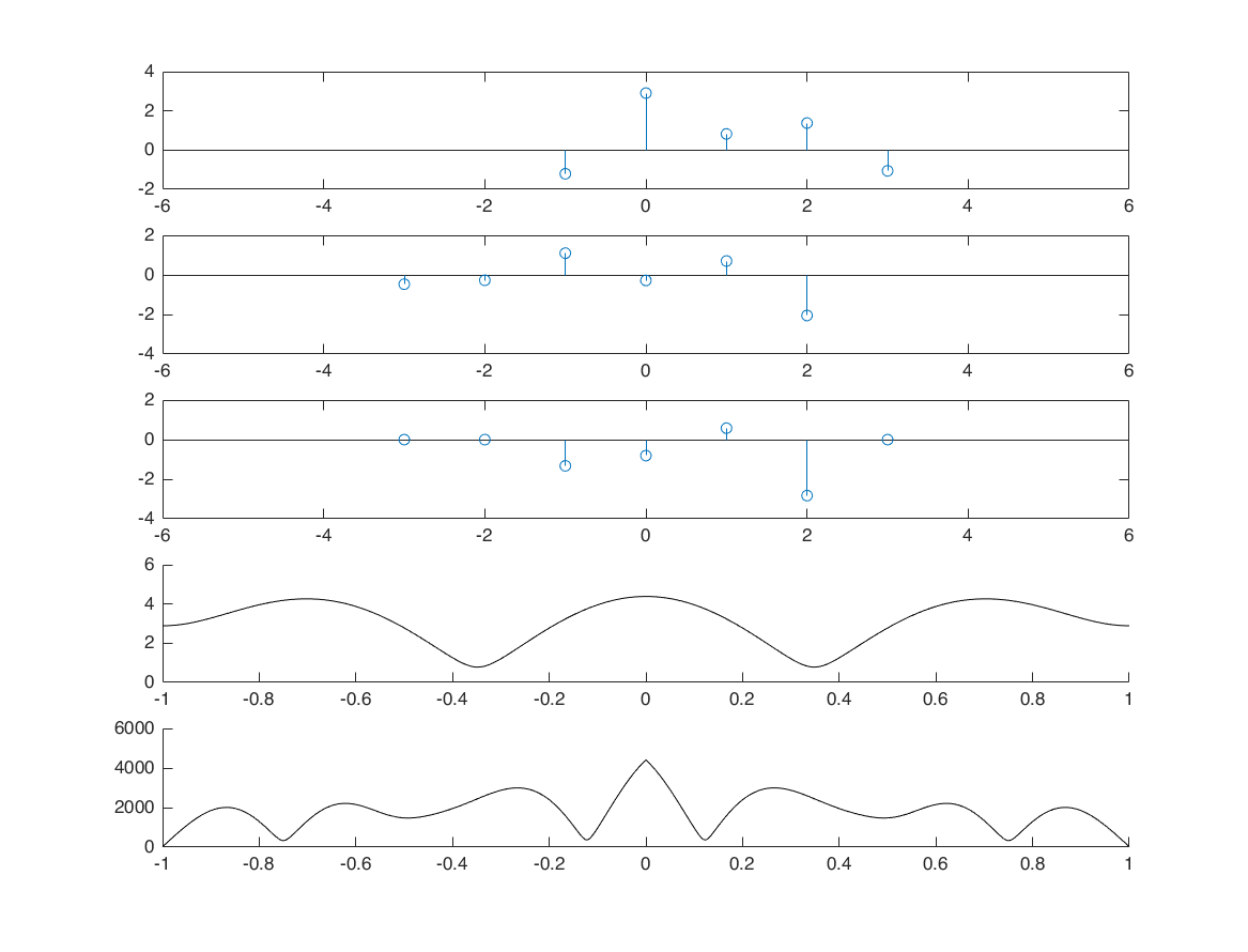
multiplication

nx1 = -1:3;
x1 = randn([1 5]);
nx2 = -3:2;
x2 = randn([1 6]);
[x3, nx3] = sigmult(x1,nx1,x2,nx2);

% define frequency axis
M = 500;
k = -M:M;
w = (pi/M)*k;

X1 = x1*(exp(-1i*pi/M)).^(nx1'*k);
X2 = x2*(exp(-1i*pi/M)).^(nx2'*k);
X3 = x3*(exp(-1i*pi/M)).^(nx3'*k);
[XX3,wp] = conv_m(X1,k,X2,k);

figure;
subplot(5,1,1); stem(nx1,x1); xlim([-6 6]);
subplot(5,1,2); stem(nx2,x2); xlim([-6 6]);
subplot(5,1,3); stem(nx3,x3); xlim([-6 6]);

subplot(5,1,4); hold on;
plot(w/pi, abs(X3), 'k');

subplot(5,1,5); hold on;
plot(wp/1000, abs(XX3), 'k');

% Question: why the 4th and 5th plots are different? Why the 5th plot has
% a larger range than the 4th plot?

Parseval's Theorem (energy)

nx = -1:3;
x = randn([1,5]);

E1 = sum(x.^2);

M = 100;
k = -M:M;
w = (pi/M)*k;
X = x*(exp(-1i*pi/M)).^(nx'*k);

E2 = trapz(abs(X).^2)*(pi/M)/(2*pi);
% we multiply the trapz integral result with (pi/M), because trapz computes
% an approximation of the integral of Y via the trapezoidal method (with unit spacing)
% thus, to create dw with pi/M spacing, we multiply it by pi/M.

disp(['Energy in time domain: ', num2str(E1)])
disp(['Energy in frequency domain: ', num2str(E2)])

Energy in time domain: 3.6282
Energy in frequency domain: 3.6282

Published with MATLAB® R2016b